


Sommaire
- Le 6 Sigma et l'Excellence Opérationnelle. Juste du bon sens ?
- Combien de valeurs sont nécessaires pour avoir un échantillon représentatif ?
- Exploiter la donnée pour optimiser le pilotage d'un procédé
- Statistical modeling: The need for a reliable approach to improve process knowledge and understanding
- Bayesian approach in cosmetical research : Application to a meta-analysis on the anti-pigmenting effect of vitamin C
- Comparabilité, équivalence, similarité... Comment les statistiques peuvent nous aider à en faire la démonstration. Et bientôt la fin d'un "blind test" pour les autorités de santé et les industriels
- Le maintien du statut validé, une étape du cycle de validation
- Stratégie de validation des procédés et mise en application de l'Annexe 15 des BPF et des guidances FDA. Vérification continue des procédés (CPV)
Cette question de taille d’échantillon, de nombreux industriels se la posent… Formulée de façon implicite par le passé, cette exigence apparait à présent comme parfaitement explicite dans de nombreuses références normatives.

Par exemple, la norme ISO 13485(1) exige lors de la vérification et de la validation de la conception et du développement des dispositifs médicaux : “L’organisme doit documenter les plans de validation qui comprennent les méthodes, les critères d’acceptation et, lorsqu’approprié, les techniques statistiques accompagnées d’une justification de la taille d’échantillonnage.”.
Or, il n’existe pas de formule unique, reconnue, indiscutable et applicable à toutes les études pour calculer des tailles d’échantillon. L’effectif dépend en effet de nombreux éléments, liés à l’objectif et au déroulement de chaque étude. Les industriels se sentent alors parfois démunis devant cette exigence nécessitant des connaissances statistiques solides et surtout, une rigueur dans leur application.
Par ailleurs, la représentativité d’un échantillon n’est pas uniquement liée à sa taille. Elle dépend directement de la manière dont est construit le plan expérimental, qui doit éviter d’introduire des biais de sélection.
Ainsi, derrière chaque problématique, l’industriel est tenu de répondre à un ensemble de questions afin de proposer un plan expérimental pertinent et adapté qui répondra à sa problématique, dans le respect de ses contraintes.
Cet article traite tout d’abord de la mise en place du plan expérimental, puis aborde la notion de taille d’échantillon pour les variables quantitatives et qualitatives. Des focus sont effectués sur certaines thématiques, comme par exemple la norme ISO 2859-1.
1. Le plan experimental comme base de discussion
Le choix du plan expérimental est l’élément de base par lequel démarrer ; en effet, il est essentiel de construire une matrice d’expériences qui permettra de répondre à l’objectif. Pour cela, différentes questions sont soulevées ; la démarche QQOQCCP (Quoi, Qui, Où, Quand, Comment, Combien, Pourquoi) peut être appliquée pour guider la réflexion.
1.1 Pourquoi réalise-t-on cette étude ?
C’est la question centrale à se poser : quel est l’objectif de l’étude ? Pourquoi a-t-on prévu de lancer cette étude, que cherche-t-on à montrer ? La formulation précise et correcte de l’objectif permettra de s’orienter vers l’approche statistique adéquate. Différentes familles de méthodes statistiques peuvent être utilisées, comme par exemple :
- Des méthodes descriptives, permettant de mesurer la performance d’un procédé, d’un équipement, ou d’analyser un historique de résultats…
- Des méthodes exploratoires, permettant l’étude des interactions entre les paramètres d’un procédé, ou la recherche de l’impact des paramètres d’un procédé sur un historique de résultats…
- Des méthodes décisionnelles, permettant l’évaluation de l’impact (ou du non-impact) d’un changement, la mesure de l’influence de facteurs et de leurs interactions sur une réponse…
Formuler correctement l’objectif permettra également de définir un objectif chiffré. Par exemple, lorsque l’on souhaite estimer une moyenne, il est nécessaire d’avoir une idée de la précision attendue. Ou lorsqu’une amélioration est attendue, il faut chiffrer l’ordre de grandeur de la différence que l’on va chercher à détecter.
1.2 Avec qui et quand ?
Ces questions concernent la planification et sont importantes pour que l’étude se déroule sereinement.
Le planning et le facteur humain constituent parfois des contraintes importantes dans l’élaboration du plan expérimental. Ces contraintes peuvent être directes (nombre limité d’opérateurs, de machines…) ou indirectes (choix économique de réaliser les tests sur un temps limité). Par exemple, si le technicien de laboratoire peut tester au maximum 10 échantillons par série, il est nécessaire de prévoir un plan expérimental prenant en compte un facteur série que l’on appellera facteur “bloc”.
De plus, étaler les essais dans le temps peut avoir pour conséquence la création d’un facteur de “bruit” qui rendra l’expérience moins performante. Il est alors possible que l’étude soit biaisée et devienne non concluante. Par exemple : on souhaite comparer 2 équipements HPLC. Pour cela, on teste x fois un échantillon sur le premier HPLC. La semaine suivante, on teste x fois le même échantillon sur l’autre HPLC. Si on constate un écart, est-il dû à une différence entre les 2 équipements ou à une instabilité de l’échantillon au cours du temps ? Ce plan expérimental n’est donc pas adapté : les 2 facteurs varient simultanément et sont alors appelés “confondus”.
Lorsque plusieurs contraintes de temps ou de ressources se superposent, une analyse des potentiels facteurs de confusion doit être effectuée en amont afin d’écarter ou de limiter les biais dans l’analyse.
1.3 Quoi et où ?
Derrière ce “quoi ?” se cachent 2 questions.
- Quels échantillons (quoi ?) et à quels stades (où ?)
Sur quel(s) produit(s) sera menée l’étude ? Sur quel(s) lot(s) ? Sur quel(s) stade(s) de fabrication? … Une réflexion doit être menée afin de définir la stratégie d’approche et l’évaluer en terme de risques : risque qualité, risque client, risque industriel… En effet, il est toujours préférable d’un point de vue financier de diminuer le nombre d’expériences en rationnalisant le choix des échantillons testés, mais il faut également se poser la question de la pertinence d’une approche “worst case”. Est-ce défendable d’un point de vue qualité ? Est-ce que le client peut le reprocher ? Est-ce que l’entreprise ne va pas passer à côté d’informations intéressante ? Ces réflexions doivent être partagées entre les experts produit et qualité.
- Quelle méthode de mesure ?
Il est généralement possible de mesurer de nombreuses choses sur les échantillons ! L’idée est donc de choisir la méthode de mesure la plus adaptée afin de répondre à l’objectif de l’étude. Si l’on souhaite valider l’homogénéité d’un produit, quelle(s) méthode(s) analytique(s) choisir pour décrire ce paramètre ? Dans certains cas, il est possible de retenir plusieurs outils ou méthodes de mesure, mais certains choix peuvent s’avérer plus pertinents que les autres (ex : dispersion d’un composant organique dans une solution aqueuse).
1.4 Comment ?
L’approche du “comment ?” est différente si l’étude est analytique ou numérative.
Une étude est dite analytique lorsqu’il n’existe pas de population finie et identifiée: l’analyse est effectuée sur un échantillon généralement construit pour l’étude.
Par exemple, on souhaite vérifier l’homogénéité d’une solution vrac dans une cuve. Comment sélectionner les échantillons pour être représentatif de l’ensemble de la cuve ? Cette question est ici aussi essentielle et l’industriel y répondra, entre autres, en fonction du type de cuve et des moyens qu’il a pour échantillonner sa solution.
Une étude est dite numérative lorsque qu’elle est menée à partir d’une population finie et identifiée, dans laquelle on sélectionne un échantillon.
Par exemple, on souhaite contrôler des unités fabriquées afin de s’assurer de l’absence de défauts. Comment bien sélectionner l’échantillon pour être représentatif du lot dans son ensemble ? Cette question est essentielle pour garantir la représentativité de l’échantillon et l’industriel y répondra en fonction de la taille du lot, mais également de la manière dont son lot a été fabriqué et ses stratégies d’échantillonnage possibles.
Il peut alors décider d’utiliser une approche raisonnée et rationnelle pour être représentatif, ou faire confiance au hasard : l’aléatoire est une très bonne méthode pour obtenir une bonne représentativité et il existe des tables de nombres au hasard permettant de travailler dans des conditions aléatoires maîtrisées.
La difficulté dans le hasard est qu’il est difficile à appliquer lorsqu’un facteur humain entre en jeu. De nombreuses études(2) ont démontré que le cerveau humain n’est pas capable de générer de façon correcte des nombres aléatoires. Même avec la meilleure volonté, son choix sera altéré par des biais de perception qui influenceront sa décision : biais liés à son interprétation de la situation, ses a priori, ses choix précédents, son raisonnement, sa culture… C’est pourquoi il faut toujours privilégier, dans la mesure du possible, un outil permettant de générer une vraie sélection aléatoire.
1.5 Structure du plan expérimental et combien ?
Une fois ces différentes questions abordées, la structure du plan expérimental peut être élaborée, répondant à l’objectif et tenant compte des contraintes.
A partir de ce plan expérimental et de l’objectif de l’étude, le statisticien va déduire quelle méthode statistique est la plus adaptée à la problématique.
Il pourra alors (enfin !) aborder la notion d’effectif et répondre à la question initiale : “Combien ?”
Par la suite, un postulat sera fait sur l’absence de biais apporté dans le plan expérimental.
2. Contrôles par mesure
De nombreuses normes exigent des tailles d’échantillons adaptées et demandent aux industriels de justifier leur choix. Il est en effet important de bien calculer une taille d’échantillon avant la conduite d’une étude afin d’avoir une forte chance de mettre en évidence le résultat recherché, de manière statistiquement significative. C’est ce qu’on appelle en statistique, la puissance. Une taille d’échantillon inadaptée (en général trop petite) peut avoir des conséquences sur la significativité des résultats statistiques, et donc sur les conclusions de l’étude.
La qualité de l’étude dépend donc directement du nombre d’échantillons testés (ou du nombre de tests à faire). D’autres paramètres entre également en compte : le risque d’erreur et la valeur ou différence attendue sur le critère mesuré. C’est pourquoi il n’est pas forcément nécessaire de systématiser des échantillons de grande taille. Dans certains domaines, une grande taille d’échantillon peut aussi fragiliser la faisabilité de l’étude.
2.1 La fluctuation d’échantillonnage
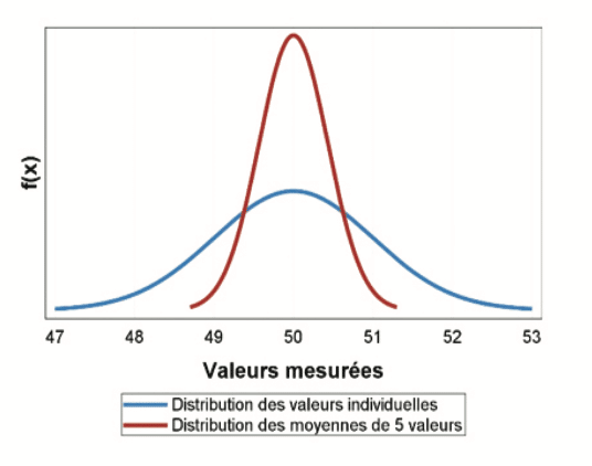
Au-delà des contraintes réglementaires évidentes, le choix d’un échantillon de taille adaptée conditionne la qualité de l’étude : plus il y aura de mesures, plus l’étude sera précise. Mais de quel niveau de précision a-t-on vraiment besoin ? L’analyse d’un échantillon donne une “estimation ponctuelle” des paramètres de la population dont il est issu ; cette estimation va changer lors de l’analyse d’un autre échantillon, mais en fluctuant toujours autour de la même tendance centrale. On appelle cela la “Fluctuation d’échantillonnage”. Par exemple, on peut mesurer 5 fois la teneur d’une solution : 50,3 – 51,2 – 50,4 – 49,1 – 48,8 ng/ml, ce qui donne une moyenne de 49,96 ng/ml. Si on effectue à nouveau 5 mesures, celles-ci vont être différentes, par exemple : 50,5 – 49,3 – 50,3 – 51,4 – 52,2 ng/mL, ce qui donne une moyenne de 50,74. La distribution des moyennes va être moins dispersée que la distribution des valeurs individuelles, et donc plus proche de la “vraie” valeur (bien que cette dernière soit rarement connue).
Le graphique ci-dessous permet d’illustrer la précision d’une moyenne de 5 valeurs (courbe rouge) sélectionnées aléatoirement dans une distribution de valeurs individuelles (courbe bleue = simulation d’une loi normale de moyenne 50 et d’écart-type 1). Ainsi, la moyenne de 5 valeurs sera généralement entre 49 et 51. Cette précision est-elle satisfaisante au vu de l’objectif de l’étude ?
On utilise généralement les intervalles de confiance pour avoir une connaissance a priori de la précision du résultat final. Par exemple, on souhaite estimer le nombre de mesures à faire pour calculer une moyenne ; on a mesuré auparavant la variabilité des résultats et l’écart-type est de 0,88. On peut utiliser la formule de l’intervalle de confiance de la moyenne pour estimer la précision en fonction du nombre de mesures :

Avec :
m0 : moyenne de l’échantillon
t : fractile de la loi de Student
α : risque d’erreur
n : taille de l’échantillon
s : écart-type de l’échantillon
Ainsi, si l’on effectue 5 tests, la moyenne fluctuera autour de sa valeur de :
± t(1-α/2 ; n-1) × s/√n = ± 2,776 × 0,88/√5 = 1,09 unités, dans 95% des cas (alpha=5%)
Si l’on effectue 10 tests, la moyenne fluctuera autour de sa valeur de :
± t(1-α/2 ; n-1) × s/√n = ± 2,262 × 0,88/√10 = 0,63 unités, dans 95% des cas (alpha=5%)
Si l’on effectue 20 tests, la moyenne fluctuera autour de sa valeur de :
± t(1-α/2 ; n-1) × s/√n = ± 2,093 × 0,88/√20 = 0,41 unités, dans 95% des cas (alpha=5%)
Plus le nombre de tests augmente, meilleure est la précision et donc l’intervalle de confiance se resserre ; cependant, le gain de précision n’est pas lié de façon linéaire au nombre de mesures.
Ainsi, l’objectif de l’étude doit clairement formuler les attentes en termes de précision du résultat recherché.
2.2 Les risques de se tromper (dit “risque d’erreur”)
Il est essentiel d’avoir à l’esprit que travailler avec un échantillon induit systématiquement deux risques de se tromper, et deux chances de prendre la bonne décision.
Le tableau suivant permet de visualiser les 4 conclusions possibles :
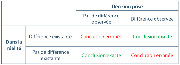
Ces risques de se tromper font intégralement partie de toute étude basée sur un échantillon ; on cherchera toujours à les limiter.
2.3 Illustration de la puissance d’un test de comparaison
Il est nécessaire de calculer a priori des tailles d’échantillons afin d’obtenir une puissance statistique suffisante. La puissance, c’est la capacité d’un test ou d’un modèle à mettre en évidence la différence recherchée, si elle existe, entre plusieurs populations.
Par exemple, si la puissance d’un plan expérimental choisi est de 50% pour une différence recherchée de 1 µg/ml, cela signifie que l’analyse de ce plan permettra de conclure à une différence significative entre les groupes seulement une fois sur deux, si cette différence est réellement de 1 µg/ml.
Ainsi, il y a une chance sur deux que le plan ne mette pas en évidence la différence de 1 µg/ml, ce qui engendre une perte de temps, d’argent, et des doutes sur l’efficacité de l’objet de l’étude.
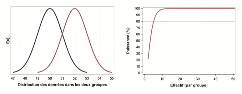
Dans le cadre d’un test de comparaison de 2 populations, un échantillon de petite taille pourra mettre en évidence des différences plutôt marquées entre les deux groupes :
En revanche, pour mettre en évidence des différences très fines entre les deux groupes, il faut nécessairement un échantillon de grande taille. Comme le montre le graphique suivant, en effectuant 50 tests dans chaque groupe, une différence de 0,5 unités ne sera détectée que dans 70% des cas :
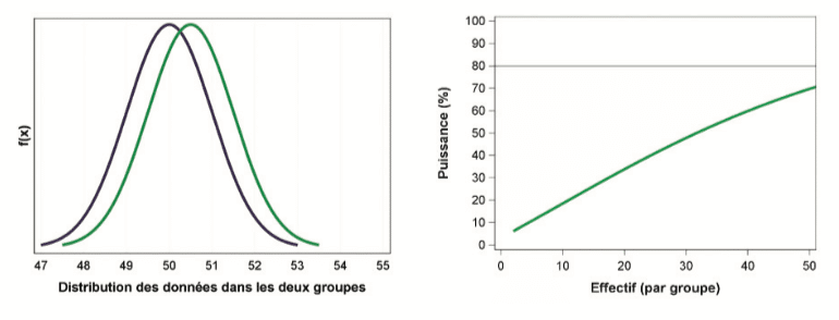
Une réflexion s’impose à présent : même en s’affranchissant de tous biais liés à la procédure d’échantillonnage et à la reproductibilité des études, quelle différence est pertinente d’un point de vue scientifique ? Est-il vraiment pertinent d’étudier un si faible effet ?
2.4 Les tests d’équivalence
Les tests statistiques ont une utilité répondant à un objectif précis. Ils doivent être utilisés dans leur contexte d’application, et à bon escient. Les tests de comparaison, couramment répandus dans les logiciels, peuvent être utilisés lorsque l’objectif de l’étude est de mettre en évidence des différences de distribution d’une mesure entre plusieurs populations.
Par exemple, lors de la comparaison d’une moyenne sur 2 groupes, et lorsque le test est significatif (par exemple, p-value = 0,01 < 0,05), cela signifie que la différence observée entre les deux moyennes lors de l’étude a 1% de chance d’être observée “par hasard”, si les deux groupes étaient issus de la même population initiale. La probabilité étant faible, on en conclut qu’il est préférable de rejeter l’hypothèse d’égalité des moyennes (H0). Lorsque la p-value est élevée, le test est non-concluant, car il ne permet pas de mettre en évidence de différence entre les deux groupes. Mais cela ne signifie pas pour autant qu’il n’y en a pas ! Cela signifie que les mesures effectuées sur cet échantillon n’ont pas permis de détecter de différence (étant données les fluctuations d’échantillonnage, une autre expérience pourrait peut-être permettre d’en détecter une).
En statistique industrielle, il est fréquent de devoir montrer l’absence d’impact d’un changement. Dans ce cas, il faut privilégier les tests d’équivalence. Ces derniers se basent sur la comparaison d’un intervalle de confiance à des bornes d’équivalence fixées.
Par exemple, lors de la comparaison de 2 moyennes, si l’intervalle de confiance de la différence est compris dans les bornes d’équivalence, il est possible de conclure à l’équivalence :
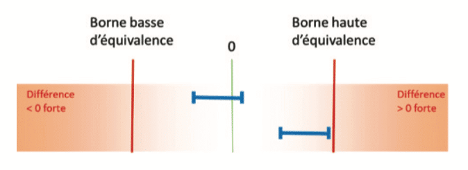
En revanche, si l’intervalle de confiance de la différence coupe l’une des bornes d’équivalence, l’échantillon ne permettra pas de conclure à l’équivalence :

Mais cela ne signifie pas pour autant qu’il y a une différence ! Cela signifie que les mesures effectuées sur cet échantillon n’ont pas permis de mettre en évidence l’équivalence (étant données les fluctuations d’échantillonnage, une autre expérience pourrait peut-être permettre de la démontrer).
La difficulté des tests d’équivalence réside dans le choix de bornes d’équivalence adaptées. Elles sont fondamentales car impactent directement le résultat du test statistique. Elles doivent être fixées au regard de la connaissance que l’industriel a sur ses méthodes, son procédé, ainsi que sur le risque industriel, client et qualité. Comme pour un test de comparaison, le calcul de la puissance du test d’équivalence est fortement recommandé.
2.5 Les autres outils
Dans un objectif exploratoire, il faut se poser la question de la pertinence de l’utilisation systématique des tests statistiques. La “preuve statistique” n’est pas forcément apportée par une p-value ; l’expert peut s’appuyer sur des outils descriptifs tels que les Boxplots, ou mesurer la force de l’effet via des mesures d’effect size(3). Ainsi, en combinant les outils statistiques avec son expertise métier et son recul de la situation, il pourra en tirer des conclusions solides, basées sur son expérience et non uniquement sur un échantillon dont les résultats pourraient être remis en cause lors d’une nouvelle expérience (cette fameuse fluctuation d’échantillonnage…).
Enfin, les méthodes bayésiennes remettent également en cause l’utilisation systématique de la p-value, propre à chacune des études. Là où l’approche fréquentiste s’appuie sur une estimation ponctuelle d’un paramètre, l’approche bayésienne consiste à s’appuyer sur un ensemble de connaissances déjà disponible sur l’objet d’étude (issue de la littérature ou d’une étude pilote, chacune restant sujette aux fluctuations d’échantillonnage). Cet ensemble de connaissances permet d’estimer une distribution a priori des données déjà connues, puis de la combiner aux résultats obtenus de la nouvelle étude menée afin d’obtenir une distribution a posteriori qui sera utilisée pour estimer des probabilités et des intervalles de crédibilité… La difficulté de cette approche consiste à identifier les études de qualité ayant été réalisées auparavant sur le sujet afin de définir la distribution a priori, celle-ci ayant un impact plus ou moins fort sur les résultats finaux.
3. Contrôle par attributs : intérêt et limite de la norme ISO 2859-1
Le contrôle par attribut consiste à noter la présence ou l’absence d’une caractéristique pour chaque pièce. Par exemple, la présence de défauts sur des unités conditionnées.
La norme ISO 2859-1(4) est alors vue par beaucoup comme une référence en termes d’effectifs d’échantillonnage, mais dans quels cas peut-elle être utilisée ? Quels sont ses apports, mais surtout, quelles sont ses limites ?
3.1 Explication de la norme ISO 2859-1
La norme ISO 2859-1(4) (ou son équivalent américain ANSI/ASQ Z1.4–2003) s’applique pour contrôler des séries continues de lots. En fonction de la taille du lot, elle indique l’effectif de l’échantillon à contrôler, ainsi que les critères à appliquer.
Mais avant d’appliquer les guidelines de cette norme, il est nécessaire de se positionner sur un certain nombre de points :
- Quel niveau de contrôle choisir ? Le niveau II, souvent utilisé par défaut, ou un autre niveau ?
- Est-ce que l’on souhaite faire un échantillonnage simple, double, multiple ?
- Quel Niveau de Qualité Acceptable (seuil NQA) choisir ?
Le choix du NQA est évidemment l’élément essentiel dans la mise en place d’un contrôle par attribut. Il doit être fixé avec la plus grande vigilance, en fonction du risque client (afin de ne pas libérer à tort des lots qui ne seraient pas acceptables pour le client) mais également en fonction du risque fournisseur (est-on capable de produire avec un très haut niveau de qualité ?). Afin de fixer ce NQA, il est indispensable de consulter les risques clients et risques fournisseurs donnés à la fin de la norme. Il est également possible de s’appuyer sur les courbes d’efficacité qui donnent une vision plus dynamique de la performance du plan de contrôle (courbes présentant la probabilité d’acceptation du lot en fonction du pourcentage de défauts dans le lot).
Par exemple, en échantillonnage simple, contrôle normal, pour un échantillon de 125 unités (lettre-code K) et un NQA de 1, le tableau indique qu’il est possible d’accepter jusqu’à 3 défauts. A partir de 4 défauts, le lot doit être refusé. Le tableau des valeurs calculées des courbes d’efficacité pour la lettre-code K indique les informations suivantes :
- Pour une probabilité d’acceptation de 95%, le taux de défaut dans le lot est de 1,1%. Cela signifie qu’un lot présentant 1,1 % de défaut sera accepté dans 95% des cas.
- Pour une probabilité d’acceptation de 50%, le taux de défaut dans le lot est de 2,9%. Cela signifie qu’un lot présentant 2,9 % de défaut sera accepté une fois sur 2.
- Pour une probabilité d’acceptation de 10%, le taux de défaut dans le lot est de 5,3%. Cela signifie qu’un lot présentant 5,3 % de défaut sera accepté dans moins de 10% des cas. Ce chiffre se retrouve également dans le tableau de la Qualité du risque client en contrôle normal.
On ne connait bien évidemment pas la quantité de défauts dans les lots. Mais cette courbe d’efficacité nous renseigne sur des informations essentielles : entre 1,1 et 5,3 % de défauts, il y aura une incertitude sur l’acceptation ou non du lot, et le lot sera généralement refusé s’il présente plus de 5,3% de défauts. Etant donné ces informations, il s’agit de savoir si ces chiffres sont en accord avec les exigences qualité du procédé.
A noter qu’il faut également prendre en compte la sévérité des contrôles. Lorsque les tests en contrôle normal montrent un niveau de qualité insuffisant, il est nécessaire de passer en contrôle renforcé. Les règles de changement de niveaux de sévérité font pleinement partie des procédures d’échantillonnage, et sont obligatoires.
3.2 Limites à l’application de cette norme
Lors d’opérations de qualification d’équipements ou de validation de procédés (validation du conditionnement, de la mise sous forme pharmaceutique…), il faut parfois démontrer que l’équipement (ou le procédé) est capable de produire des unités présentant un faible nombre de défauts. Cette norme, pourtant très informative, n’est pas un outil recommandé pour déterminer l’effectif qui permettra de prouver que le niveau de qualité est celui attendu.
La première raison est liée au champ d’utilisation de cette norme : elle spécifie l’échantillonnage pour l’acceptation ou la non-acceptation de lots, lors de contrôles par attributs d’une série continue de lots. Cette norme n’est initialement pas adaptée pour des lots isolés, même s’il est toléré de l’utiliser en consultant les courbes d’efficacités.
De plus, il faut être conscient que la norme “accepte” des défauts : on parle de NQA en tant que Niveau de Qualité Acceptable. Parfois, certains industriels font le choix de se positionner au niveau de contrôle “le plus sévère”. En pratique, cela se traduit par un contrôle de 2000 échantillons avec un NQA fixé à 0.01 et le refus du lot s’il y a 1 défaut. Si l’industriel fait au contraire le choix d’accepter le lot, cela signifie qu’il juge acceptable d’observer 1 défaut sur 10 000, en moyenne. Dans le cadre d’une opération de qualification ou de validation, ce positionnement est discutable. Il serait en effet plus pertinent d’estimer la proportion de défauts dans le lot, et de fixer une limite acceptable en fonction des performances du procédé, des exigences qualité, et des attentes internes ou externes.
3.3 Alors, que faire ? Mesurer les performances du procédé
L’approche proposée ci-dessous est une approche conservative pouvant être retenue.
Des essais préliminaires sont nécessaires afin de comprendre les variations potentielles sur la mesure de la performance et ainsi juger du niveau de maitrise actuel. Une fois de plus, afin d’évaluer la performance du procédé, il s’agit de déterminer combien d’échantillons seront nécessaires pour juger la performance. Les intervalles de confiance sont encore un bon outil pour répondre à cet objectif. Il est en effet possible d’utiliser la formule conservative de l’intervalle de confiance de Clopper and Pearson(5)
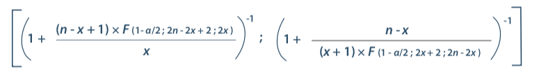
Avec :
n : nombre total de valeurs
x : nombre de réponses positives
α : risque d’erreur
F : loi de Fisher
Par exemple, on considère une mireuse automatique avec un taux de détection garanti par le fabricant supérieur à 90%.
Est-ce que 100 échantillons sont suffisants pour tester la machine ? L’intervalle de confiance bilatéral à 95% de 90,0% est [82,4% ; 95,1%]. Cela signifie que si l’on effectue plusieurs fois des tests sur 100 échantillons, les proportions seront généralement trouvées entre 82,4% et 95,1%. Si l’on obtient un pourcentage supérieur à 95,1%, cela signifie que le taux de détection est supérieur à 90,0% (au risque de se tromper dans 2,5% des cas). A l’inverse, si l’on obtient un pourcentage inférieur à 82,4%, cela signifie que le taux de détection est inférieur à 90,0% (au risque de se tromper dans 2,5% des cas).
Ainsi, si 100 échantillons défectueux sont testés, le critère d’acceptabilité peut être d’obtenir au moins 96 unités défectueuses détectées, afin de garantir un taux de détection de 90%. Si ce critère parait trop restrictif, il est bien évidemment possible d’augmenter la taille de l’échantillon, car cela diminue l’intervalle de confiance, et rend le critère plus accessible.
Conclusion
La taille d’échantillon est souvent une question centrale dans les études statistiques ; Pour mettre en place une étude pertinente et adaptée, il faut nécessairement formuler clairement l’objectif, puis définir la structure du plan expérimental qui pourra être appliqué. Par la suite, la notion d’effectif pourra être abordée.
Que le paramètre mesuré soit qualitatif ou quantitatif, des outils statistiques (tels que les intervalles de confiance ou la puissance, entre autres) permettent de s’assurer que l’effectif choisi répondra à l’objectif avec un risque connu. Ces outils statistiques doivent être compris pour être utilisés à bon escient. Chaque test statistique a un domaine d’application précis, et doit être utilisé dans ce cadre.
Comme tout outil, pour qu’ils soient utiles et performants, il faut qu’ils soient utilisés conformément à leurs objectifs et dans le respect de leurs conditions d’application ; mais il faut également que la personne qui les utilise apporte son savoir-faire, son expertise et sa connaissance. Ainsi, c’est la combinaison des compétences de l’utilisateur et de l’adéquation de l’outil qui fera la pertinence de l’étude.
Merci à ceux ayant contribué à la rédaction de cet article : Marine Ragot, Marine Dufournet, Françoise Guérillot-Maire, Florian Kroell, Laura Turbatu, François Conesa.
Partager l’article


Catherine TUDAL – SOLADIS
ctudal@soladis.fr
Bibliographie
(1) “norme internationale de gestion de la qualité des dispositifs médicaux” ISO 13485, avril 2016
(2) “Logique et Calcul – Le hasard géométrique n’existe pas !” Pour la science – n° 341 mars 2006
(3) “Pvalues, the ‘gold standard’ of statistical validity, are not as reliable as many scientists assume” Nature, 13 février 2014
(4) “Règles d’échantillonnage pour les contrôles par attributs” NF ISO 2859-1, avril 2000
(5) “Statistical Intervals A Guide for Practitioners” Gérald J. HAHN and William Q. MEEKER, 1991
